Component - GDSFactory

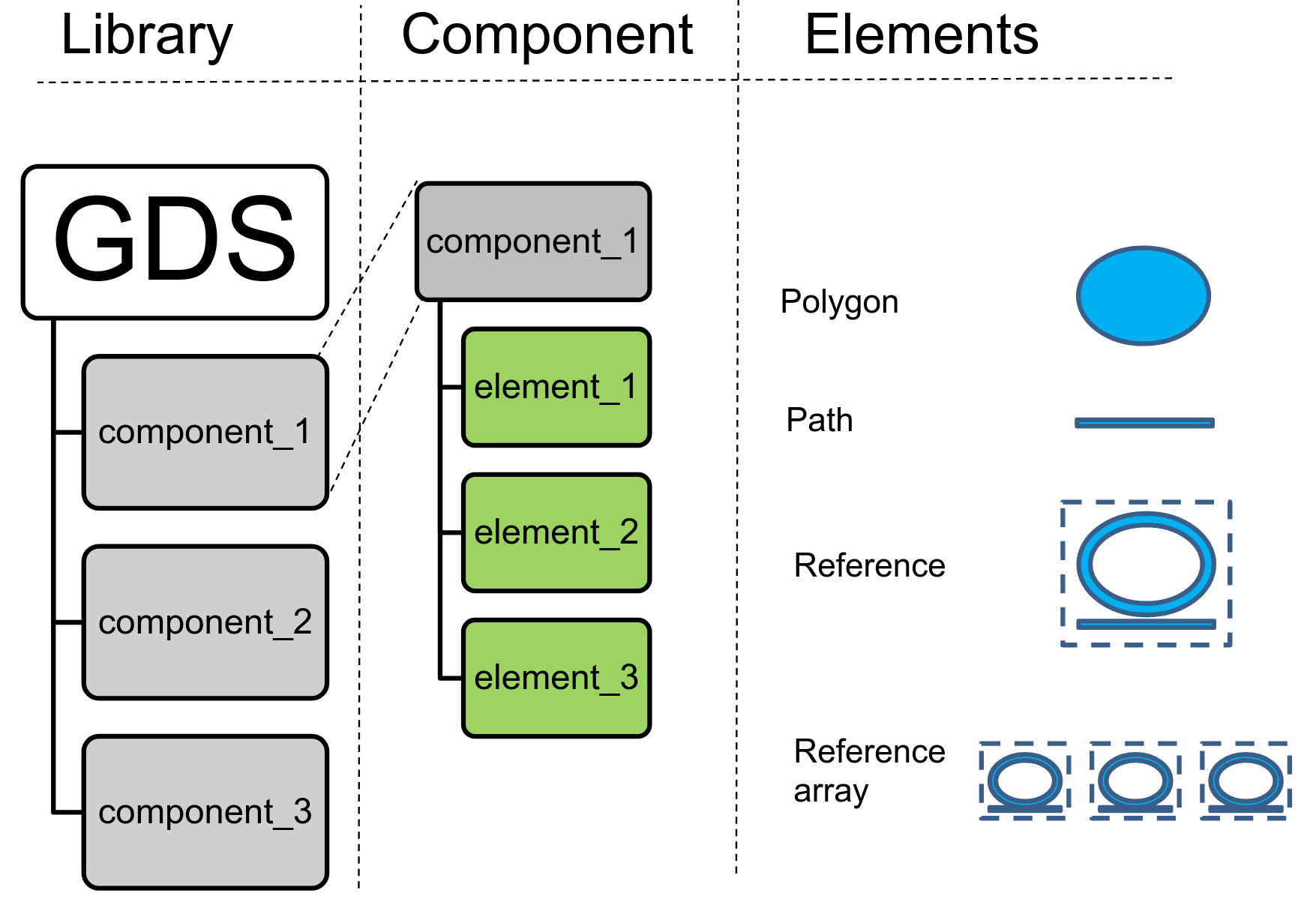
A Component is like an empty canvas, where you can add polygons, references to other Components and ports (to connect to other components)

In gdsfactory all dimensions are in microns

Polygons¶

You can add polygons to different layers. By default all units in gdsfactory are in um.

import gdsfactory as gf

# Create a blank component (essentially an empty GDS cell with some special features)
c = gf.Component()
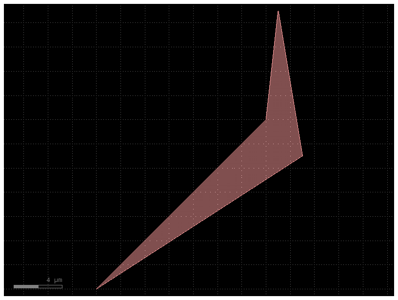
p1 = c.add_polygon([(-8, -6), (6, 8), (7, 17), (9, 5)], layer=(1, 0))
c.write_gds("demo.gds")  # write it to a GDS file. You can open it in klayout.
c.show()  # show it in klayout
c.plot()  # plot it in jupyter notebook

2025-04-21 12:50:01.699 | WARNING  | kfactory.kcell:show:3520 - Could not connect to klive server

Exercise :

Make a component similar to the one above that has a second polygon in layer (2, 0)

c = gf.Component()

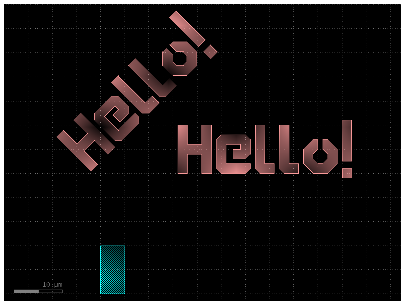
# Create some new geometry from the functions available in the geometry library
t = gf.components.text("Hello!")
r = gf.components.rectangle(size=(5, 10), layer=(2, 0))

# Add references to the new geometry to c, our blank component
text1 = c.add_ref(t)  # Add the text we created as a reference
# Using the << operator (identical to add_ref()), add the same geometry a second time
text2 = c << t
r = c << r  # Add the rectangle we created

# Now that the geometry has been added to "c", we can move everything around:
text1.movey(25)
text2.move((5, 30))
text2.rotate(45)
r.movex(-15)

print(c)
c.plot()

Component(name=Unnamed_1, ports=[], instances=['text_gdsfactorypcompone_6de68a3d_0_25000', 'text_gdsfactorypcompone_6de68a3d_-17678_24749', 'rectangle_gdsfactorypco_73f90021_-15000_0'], locked=False, kcl=DEFAULT)

c = gf.Component()
p1 = gf.kdb.DPolygon([(-8, -6), (6, 8), (7, 17), (9, 5)])  # DPolygons are in um
p2 = p1.sized(2)

c.add_polygon(p1, layer=(1, 0))
c.add_polygon(p2, layer=(2, 0))
c.plot()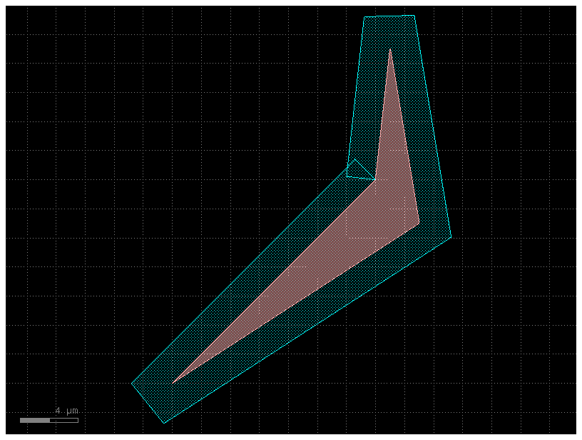

For operating boolean operations Klayout Regions are very useful.

Notice that Many Klayout objects are in Database Units (DBU) which usually is 1nm, therefore we need to convert a DPolygon (in um) to DBU.

c = gf.Component()
p1 = gf.kdb.DPolygon([(-8, -6), (6, 8), (7, 17), (9, 5)])
r1 = gf.Region(p1.to_itype(gf.kcl.dbu))  # convert from um to DBU
r2 = r1.sized(2000)  # in DBU
r3 = r2 - r1

c.add_polygon(r3, layer=(2, 0))
c.plot()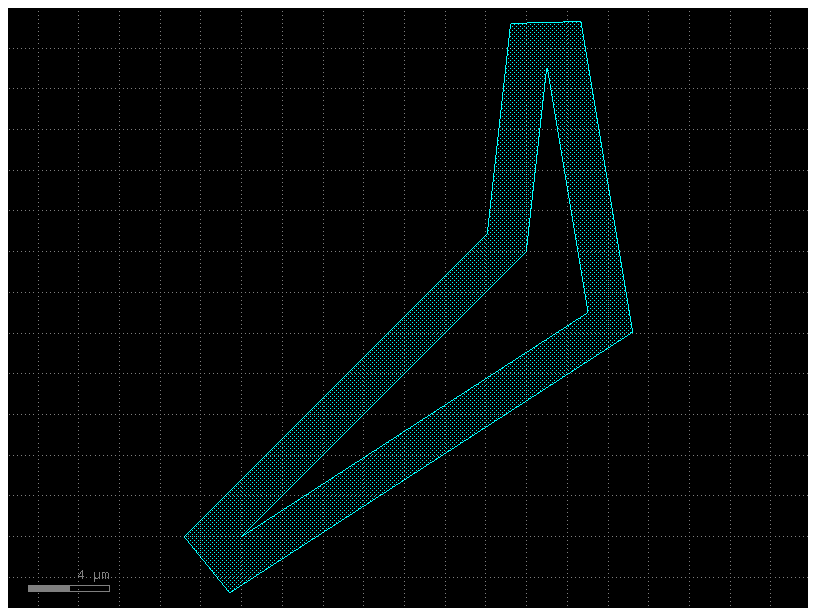

c = gf.Component()
p1 = [(-8, -6), (6, 8), (7, 17), (9, 5)]
s1 = c.add_polygon(p1, layer=(1, 0))
r1 = gf.Region(s1.polygon)
r2 = r1.sized(2000)  # in DBU, 1 DBU = 1 nm, size it by 2000 nm = 2um
r3 = r2 - r1
c.add_polygon(r3, layer=(2, 0))
c.plot()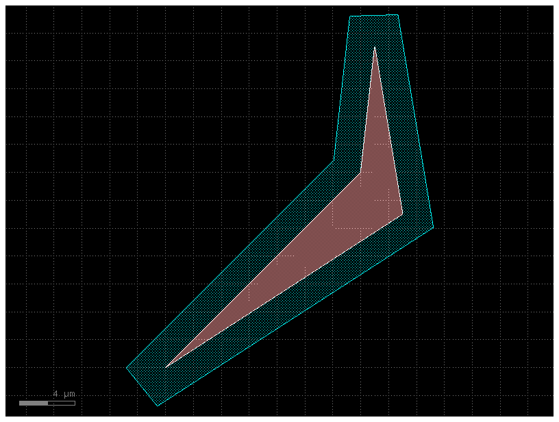

Connect ports¶

Components can have a “Port” that allows you to connect ComponentReferences together like legos.

You can write a simple function to make a rectangular straight, assign ports to the ends, and then connect those rectangles together.

Notice that connect transform each reference but things won’t remain connected if you move any of the references afterwards.

def straight(length=10, width: float = 1, layer=(1, 0)):
    c = gf.Component()
    c.add_polygon([(0, 0), (length, 0), (length, width), (0, width)], layer=layer)
    c.add_port(
        name="o1", center=(0, width / 2), width=width, orientation=180, layer=layer
    )
    c.add_port(
        name="o2", center=(length, width / 2), width=width, orientation=0, layer=layer
    )
    return c


c = gf.Component()

wg1 = c << straight(length=6, width=2.5, layer=(1, 0))
wg2 = c << straight(length=6, width=2.5, layer=(2, 0))
wg3 = c << straight(length=15, width=2.5, layer=(3, 0))
wg2.movey(10)
wg2.rotate(10)

wg3.movey(20)
wg3.rotate(15)

c.plot()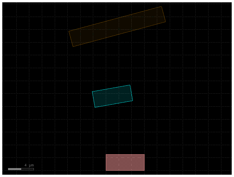

wg2.movex(10)

Unnamed_9: ports ['o1', 'o2'], KCell(name=Unnamed_11, ports=['o1', 'o2'], instances=[], locked=False, kcl=DEFAULT)

Now we can connect everything together using the ports:

Each straight has two ports: ‘o1’ and ‘o2’, respectively on the East and West sides of the rectangular straight component. These are arbitrary names defined in our straight() function above

# Let's keep wg1 in place on the bottom, and connect the other straights to it.
# To do that, on wg2 we'll grab the "o1" port and connect it to the "o2" on wg1:
wg2.connect("o1", wg1.ports["o2"], allow_layer_mismatch=True)

# Next, on wg3 let's grab the "o1" port and connect it to the "o2" on wg2:
wg3.connect("o1", wg2.ports["o2"], allow_layer_mismatch=True)

c.plot()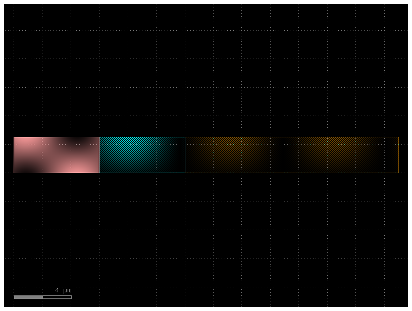

Ports can be added by copying existing ports. In the example below, ports are added at the component-level on c from the existing ports of children wg1 and wg3 (i.e. eastmost and westmost ports)

c.add_port("o1", port=wg1.ports["o1"])
c.add_port("o2", port=wg3.ports["o2"])
c.plot()

You can show the ports by adding port pins with triangular shape or using the show_ports plugin

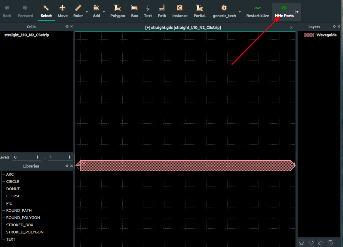
c.draw_ports()
c.plot()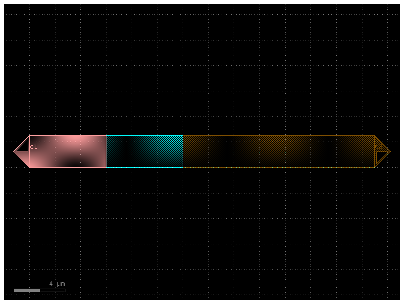

Also you can visualize ports in klayout as the ports are stored in the GDS cell metadata.

Move and rotate Instances¶

You can move, rotate, and reflect component instances.

There are two main types of movement:

Using Integer DataBaseUnits (DBU) (default), in most foundries, 1 DBU = 1nm
Using Decimals Floats. Where 1.0 represents 1.0um

c = gf.Component()

wg1 = c << straight(length=1, layer=(1, 0))
wg2 = c << straight(length=2, layer=(2, 0))
wg3 = c << straight(length=3, layer=(3, 0))

# Shift the second straight we created over by dx = 2, dy = 2 um. D stands for Decimal
wg2.move((2.0, 2.0))

# Then, move again the third straight by 3um
wg3.movex(3)  # equivalent to wg3.move(3)

c.plot()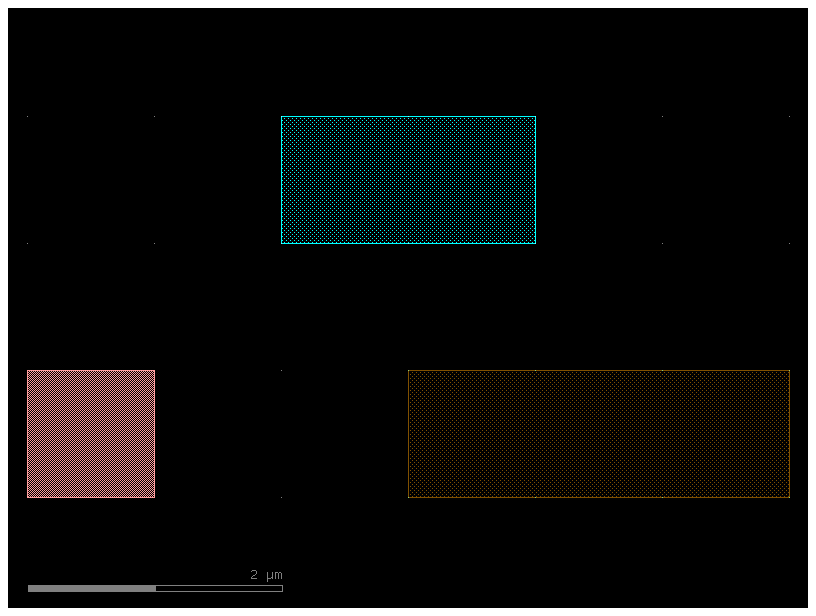

You can also define the positions relative to other references.

c = gf.Component()

wg1 = c << straight(length=1, layer=(1, 0))
wg2 = c << straight(length=2, layer=(2, 0))
wg3 = c << straight(length=3, layer=(3, 0))

# Shift the second straight we created over so that the xmin matches wg1.xmax
wg2.xmin = wg1.xmax

# Then, leave a 1um gap with on the last straight
wg3.xmin = wg2.xmax + 1

c.plot()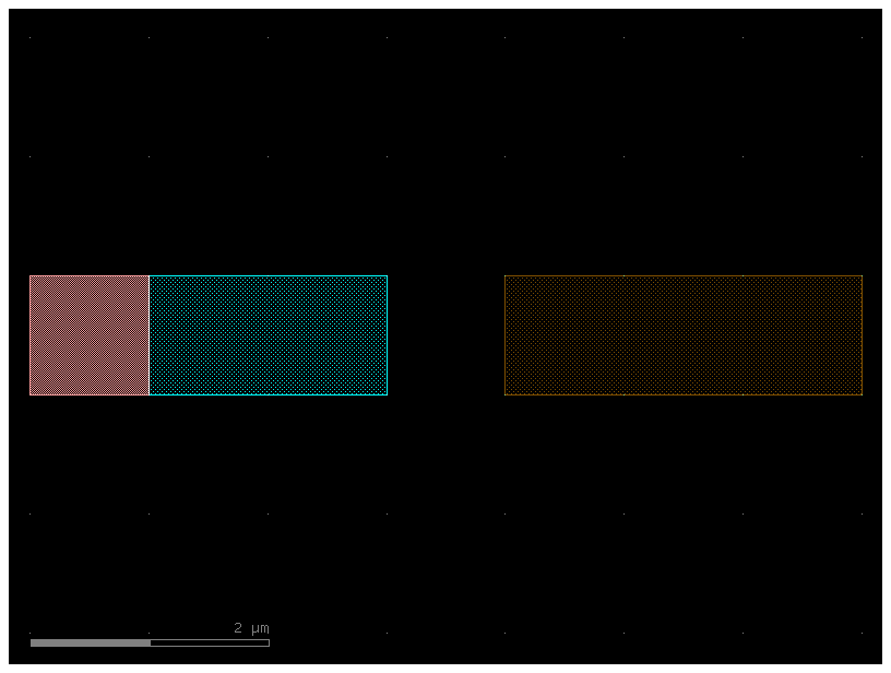

Ports¶

Your straights wg1/wg2/wg3 are references to other waveguide components.

If you want to add ports to the new Component c you can use add_port, where you can create a new port or use a reference to an existing port from the underlying reference.

You can access the ports of a Component or ComponentReference

import gdsfactory as gf


def straight(length: float = 10, width: float = 1, layer=(1, 0)):
    c = gf.Component()
    c.add_polygon([(0, 0), (length, 0), (length, width), (0, width)], layer=layer)
    c.add_port(
        name="o1", center=(0, width / 2), width=width, orientation=180, layer=layer
    )
    c.add_port(
        name="o2", center=(length, width / 2), width=width, orientation=0, layer=layer
    )
    return c

s = straight(length=10)
s.draw_ports()
s.pprint_ports()
s

References¶

Now that your component c is a multi-straight component, you can add references to that component in a new blank Component c2, then add two references and shift one to see the movement.

c2 = gf.Component()
wg1 = straight(length=10)
wg2 = straight(length=10, layer=(2, 0))
mwg1_ref = c2.add_ref(wg1)
mwg2_ref = c2.add_ref(wg2)
mwg2_ref.movex(10)
c2.plot()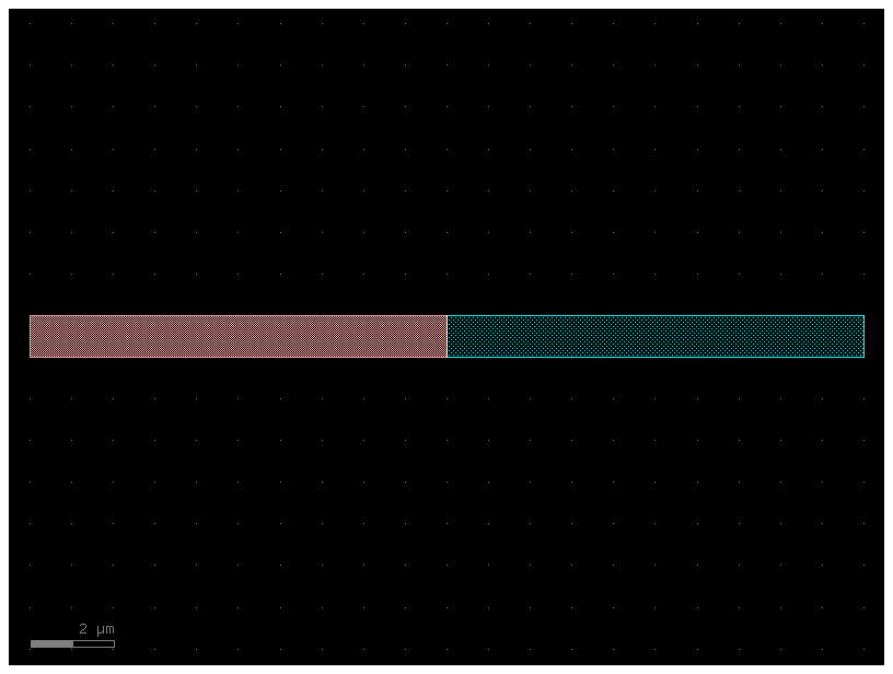

# Like before, let's connect mwg1 and mwg2 together
mwg1_ref.connect(port="o2", other=mwg2_ref.ports["o1"], allow_layer_mismatch=True)
c2.plot()

Labels¶

You can add abstract GDS labels to annotate your Components, in order to record information directly into the final GDS file without putting any extra geometry onto any layer This label will display in a GDS viewer, but will not be rendered or printed like the polygons created by gf.components.text().

c2.add_label(text="First label", position=mwg1_ref.dcenter)
c2.add_label(text="Second label", position=mwg2_ref.dcenter)

# labels are useful for recording information
c2.add_label(
    text=f"The x size of this\nlayout is {c2.xsize}",
    position=(c2.x, c2.y),
    layer=(10, 0),
)
c2.plot()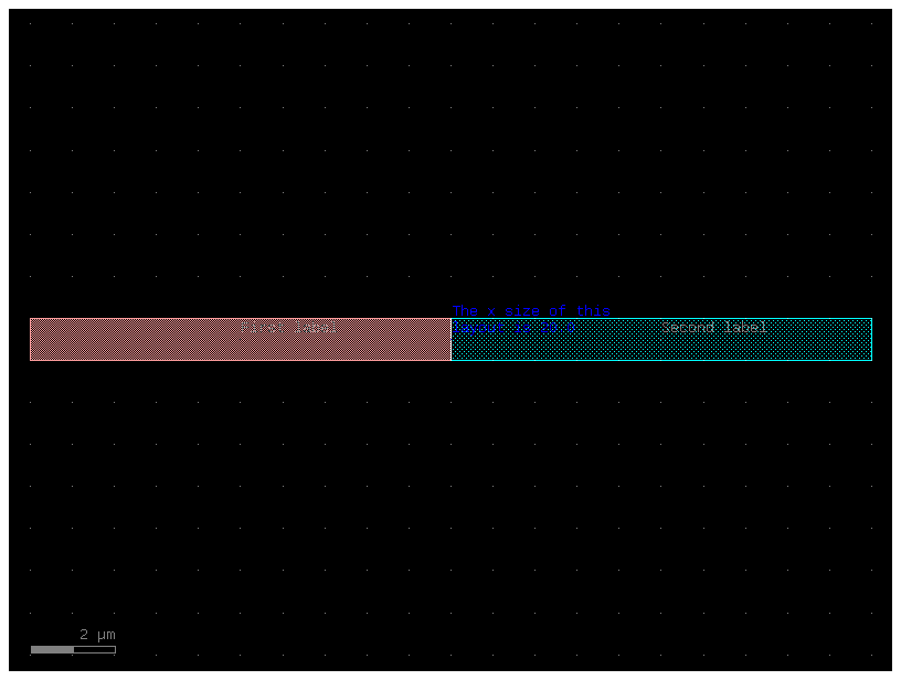

Another simple example

c = gf.Component()
r = c << gf.components.rectangle(size=(1, 1))
r.x = 0
r.y = 0
c.add_label(
    text="Demo label",
    position=(0, 0),
    layer=(1, 0),
)
c.plot()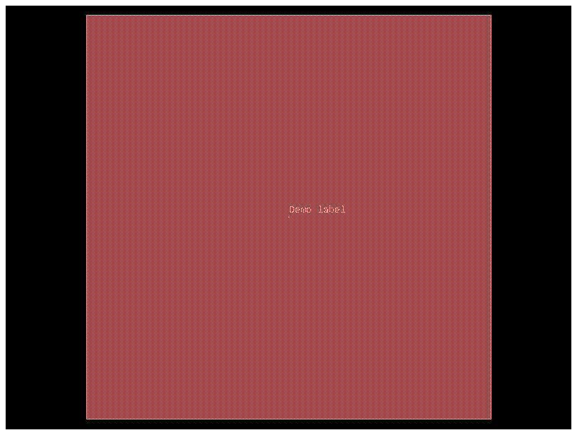

Boolean shapes¶

If you want to subtract one shape from another, merge two shapes, or perform an XOR on them, you can do that with the boolean() function.

The operation argument should be {not, and, or, xor, ‘A-B’, ‘B-A’, ‘A+B’}. Note that ‘A+B’ is equivalent to ‘or’, ‘A-B’ is equivalent to ‘not’, and ‘B-A’ is equivalent to ‘not’ with the operands switched

c = gf.Component()
e1 = c.add_ref(gf.components.ellipse(layer=(2, 0)))
e2 = c.add_ref(gf.components.ellipse(radii=(10, 6), layer=(2, 0))).movex(2)
e3 = c.add_ref(gf.components.ellipse(radii=(10, 4), layer=(2, 0))).movex(5)
c.plot()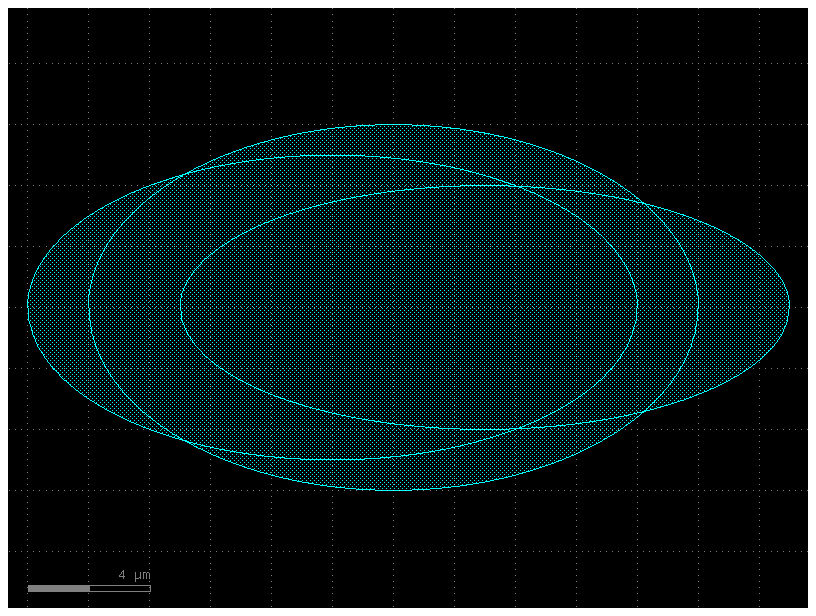

c2 = gf.boolean(A=e2, B=e1, operation="not", layer=(2, 0))
c2.plot()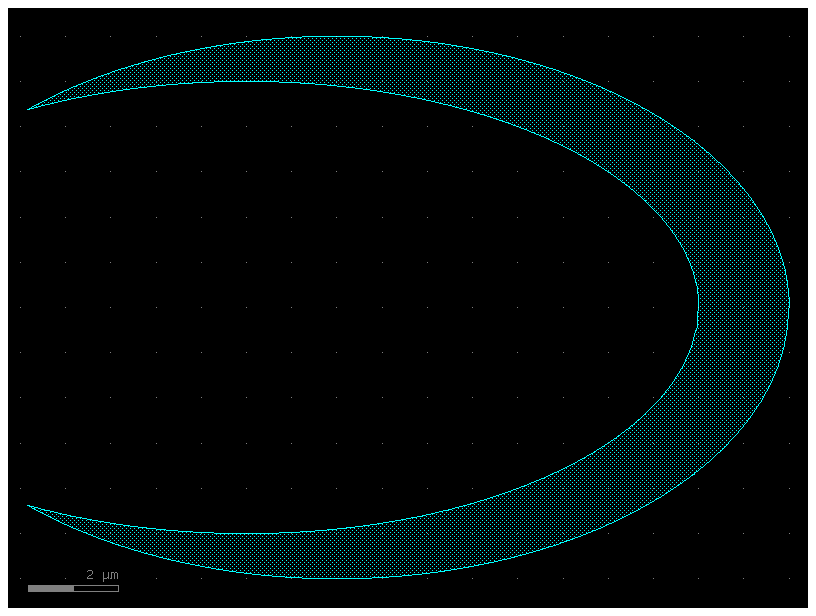

Move Reference by port¶

c = gf.Component()
mmi = c.add_ref(gf.components.mmi1x2())
bend = c.add_ref(gf.components.bend_circular(layer=(1, 0)))
c.plot()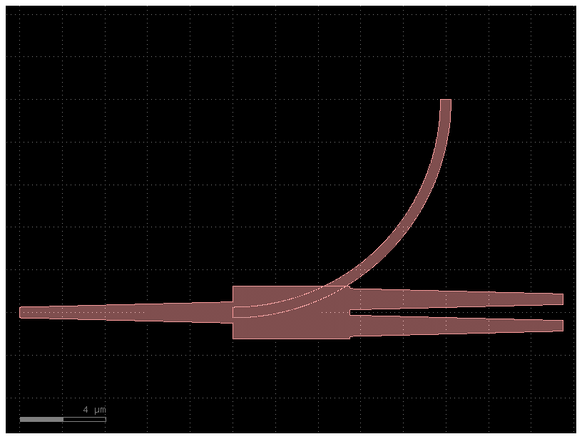

bend.connect("o1", mmi.ports["o2"])  # connects follow Source -> Destination syntax
c.plot()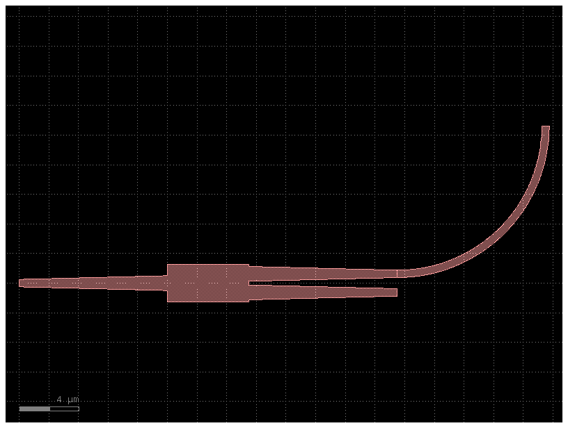

Mirror reference¶

By default the mirror works along the y-axis.

c = gf.Component()
mmi = c.add_ref(gf.components.mmi1x2())
bend = c.add_ref(gf.components.bend_circular())
bend.connect(
    "o1", mmi.ports["o2"], mirror=True
)  # connects follow Source -> Destination syntax
c.plot()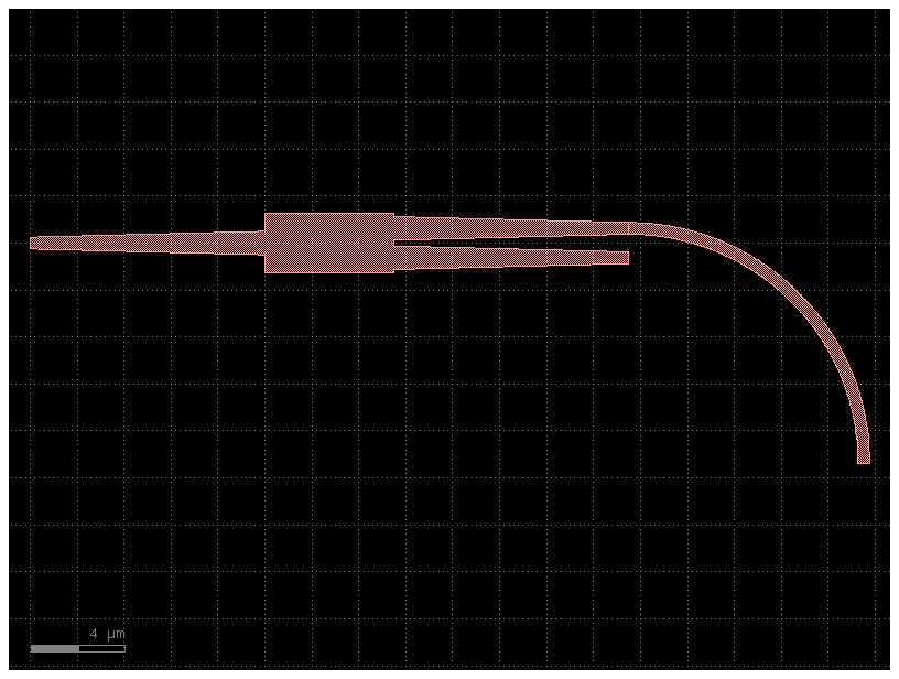

Write¶

You can write your Component to:

GDS file (Graphical Database System) or OASIS for chips.
gerber for PCB.
STL for 3d printing.

import gdsfactory as gf

c = gf.components.cross()
c.write_gds("demo.gds")
c.plot()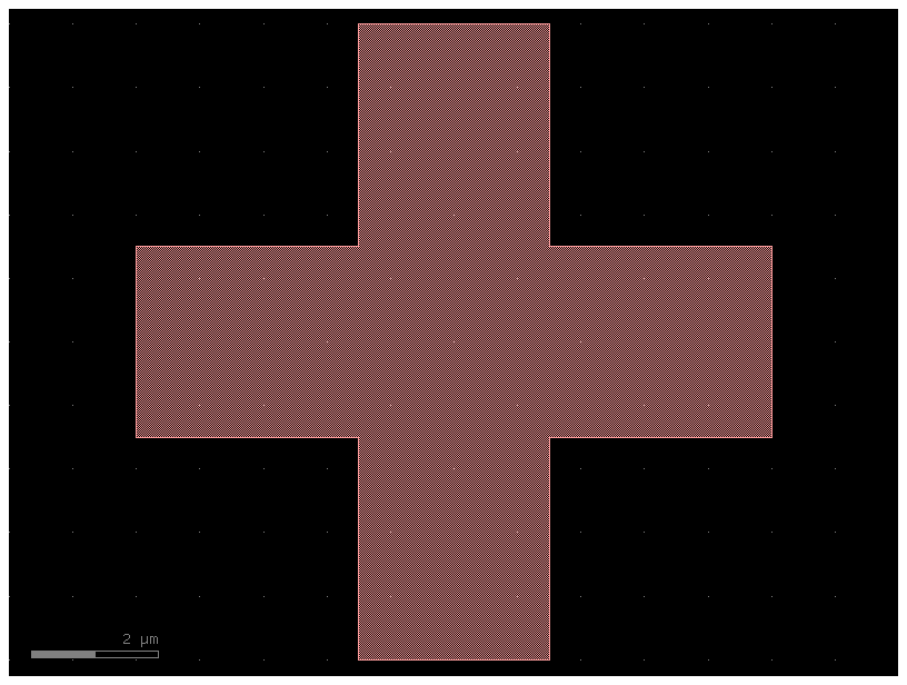

You can see the GDS file in Klayout viewer.

Sometimes you also want to save the GDS together with metadata (settings, port names, widths, locations ...) in YAML.

c.write_gds("demo.gds", with_metadata=True)

PosixPath('demo.gds')

⚠️ Warning!

If you plan to use Calibre DRC or Cadence in your design workflow, make sure to set:

with_metadata=False

GDSFactory stores ports and settings information inside the GDS file. However, this format may not be compatible with certain EDA tools like Calibre and Cadence. To ensure smooth integration, disable metadata when exporting your GDS files.

OASIS is a newer format that can store CAD files and that reduces the size.

c.write("demo.oas")

You can also save it as STL for 3D printing or for device level simulations. For that you need to extrude the polygons using the information in the LayerStack.

gf.export.to_stl(c, "demo.stl")

Write PosixPath('/home/runner/work/gdsfactory/gdsfactory/notebooks/demo_1_0.stl') zmin = 0.000, height = 0.220

scene = c.to_3d()
scene.show()